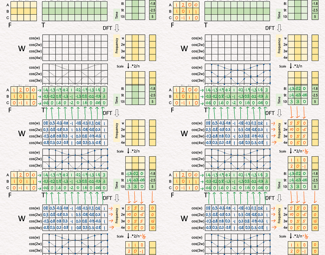
In signal processing, the Discrete Fourier Transform (DFT) is no doubt the most important method. But the math involved is extremely complex, literally, involving a summation over a complex number term e^(-iwt), where e is the Euler number, i is the imaginary unit, w is the angular frequency, and t is time.
I developed this exercise to demonstrate that underneath such complexity, DFT is just a series of matrix multiplications you can calculate by hand. ✍️ Once you see that, it should not surprise you that a deep neural network, which is also a series of matrix multiplications, with activation functions in-between, can learn to perform DFT to process and analyze signals so effectively.
How does DFT work?
Walkthrough
[1] Given
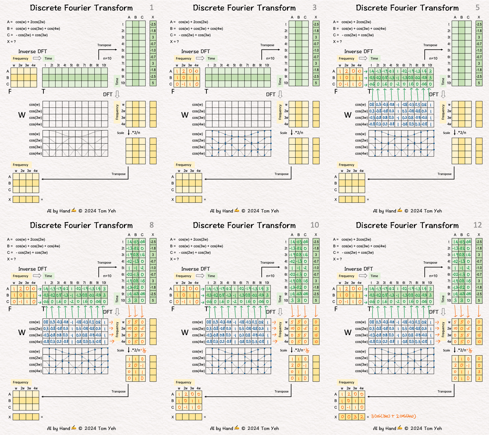
↳ Signals A, B, and C in the 🟧 frequency domain:
A = cos(w) + 2cos(2w)
B = cos(w) + cos(3w) + cos(4w)
C = -cos(2w) + cos(3w)
Each signal is a weighed sum of four cosine waves at frequencies 1w, 2w, 3w, and 4w.
We will apply Inverse DFT to convert the signals to time domain representations, and then demonstrate DFT can convert back to their original frequency domain representations.
↳ Signal X in the 🟩 time domain. X is sampled at 10 time points 1t, 2t, …, 10t:
X = [-2.5, -1.8, 3, -0.7, -1.0, -0.7, 3, -1.8, -2.5, 5]
Suppose X is also a weighted sum of the same four cosine waves, but we don’t already know their weights. We will apply DFT to discover them.
[2] 🟧 Frequency Matrix (F)
↳ Write the coefficients of A, B, C as a matrix F. Each signal is a row. Each frequency is a column.
↳ A → [1, 2, 0, 0]
↳ B → [1, 0, 1, 1]
↳ C → [0, 1-, 1, 0]
[3] Cosine → Discrete
↳ Sample from the continuous cosine waves at discrete time points 1t, 2t, 3t, to 10t.
[4] Cosine Matrix (W)
↳ Write the samples as a matrix, Each frequency is a row. Each time point is a column.
[5] Inverse DFT: 🟧 Frequency → 🟩 Time
↳ Multiply the frequency matrix F and the cosine matrix W.
↳ The meaning of this multiplication is to linearly combine the four cosine waves (rows in W) into time-domain signals (rows in T) using the weights specified in F.
↳ The result is matrix T, which are signals A, B, C converted to the time domain. Each signal is a row. Each time point is a column.
[6] Transpose
↳ Transpose T, converting each signal’s time domain representation from a row to a column.
[7] DFT: 🟩 Time → 🟧 Frequency
↳ Multiply the cosine matrix W with the transpose of matrix T.
↳ The purpose of this multiplication is to take a dot-product between each time-domain signal (columns in the transpose of T) and each cosine wave (rows in W), which has the effect of projecting the signal onto a cosine wave to determine how much they are correlated. Zero means not correlated at all.
↳ The result is an intermediate version of the “recovered” frequency matrix where each column corresponds to a signal and each row corresponds to a frequency.
↳ Compared to the original frequency matrix F, this intermediate matrix has non-zero weights in the correct places, but scaled up by a factor of 5 (n/2, n=10). For example, signal A, originally [1,2,0,0], is recovered at [5,10,0,0].
[8] Scale
↳ Multiply each value by 2/n = 1/5 to scale down the intermediate matrix to match the magnitude of the original frequency matrix F.
[9] Transpose
↳ Transpose the recovered frequency matrix back to the same orientation of the original frequency matrix F.
↳ Like magic 🪄, the result is identical to the original F, which means DFT successfully recovered the frequency components of signals A, B, C.
[10] Apply DFT to X: 🟩 Time → 🟧 Frequency
↳ Now that we have some confidence in DFT’s ability to recover frequency components, we apply DFT to X’s time-domain representation by multiplying W with X.
↳ The result is the an intermediate matrix.
[11] Scale
↳ Similarly, we scale down by a factor of 5 to obtain the recovered frequency components of X (a column).
[12] Transpose
↳ Similarly, we transpose the recovered column to row to match the orientation of the frequency matrix.
↳ Using the coefficients [0,0,3,2], we can write the equation of X as 3cos(3w) + 2cos(4w).
Notes
I hope this by hand exercise helps you understand the essence of DFT. But there is more technical details, such as:
Sine: The complete DFT math also includes sine waves that follow a similar calculation process.
Phase: Here, we assume all the cosine waves are aligned at the origin, namely, phase is 0. If a phase p is added, for example, cos(w+p), we will need to calculate the sine component and use their ratio to figure out what p is.
Magnitude: If phase is not zero, the magnitude will need to be calculated by combining both cosine and sine terms.


